Regression models forest plot

Data

We use the R dataset lung in the survival package.
The name of the variables is modified thanks to the transmute() function. This allows to display the desired names on the forest plot and to select the desired variables :

library(survival)
library(dplyr)

pretty_lung <- lung %>%
  transmute(time,
    status,
    Age = age,
    Sex = factor(sex, labels = c("Male", "Female")),
    ECOG = factor(lung$ph.ecog),
    `Meal Cal` = meal.cal
  )

pretty_lung format :

A data frame with 228 observations on the following 6 variables :
time Survival time in days
status Censoring status 1=censored, 2=dead
Age Age in years
Sex Patient sex
ECOG ECOG performance score. 0=asymptomatic, 1= symptomatic but completely ambulatory, 2= in bed <50% of the day, 3= in bed > 50% of the day but not bedbound, 4 = bedbound
Meal Cal Calories consumed at meals

#Head of dataset
knitr::kable(head(pretty_lung,8), align = "l")

time	status	Age	Sex	ECOG	Meal Cal
306	2	74	Male	1	1175
455	2	68	Male	0	1225
1010	1	56	Male	0	NA
210	2	57	Male	1	1150
883	2	60	Male	0	NA
1022	1	74	Male	1	513
310	2	68	Female	2	384
361	2	71	Female	2	538

`forestmodel` package

The forest_model function produce a forest plot based on a regression model

forest_model(
model, regression model produced by lm, glm, coxph
panels = default_forest_panels(model, factor_separate_line = factor_separate_line), list with details of the panels
covariates = NULL, a character vector optionally listing the variables to include in the plot
exponentiate = NULL, whether the numbers on the x scale should be exponentiated for plotting
funcs = NULL, optional list of functions required for formatting panels$display
factor_separate_line = FALSE, whether to show the factor variable name on a separate line
format_options = forest_model_format_options(), formatting options as a list as generated by forest_model_format_options
theme = theme_forest(), theme to apply to the plot
limits = NULL, limits of the forest plot on the X-axis
breaks = NULL, breaks to appear on the X-axis
return_data = FALSE, return the data to produce the plot as well as the plot itself
recalculate_width = TRUE, TRUE to recalculate panel widths using the current device or the desired plot width in inches
recalculate_height = TRUE, TRUE to shrink text size using the current device or the desired plot height in inches
model_list = NULL, list of models to incorporate into a single forest plot
merge_models = FALSE, if TRUE, merge all models in one section
exclude_infinite_cis = TRUE, whether to exclude points and confidence intervals that go to positive or negative infinity from plotting
...
)

Forest plot based on a Cox model

We use the function forest_model to print the forest plot :

library(survival)
library(dplyr)
library(forestmodel)

print(forest_model(coxph(Surv(time, status) ~ ., pretty_lung)))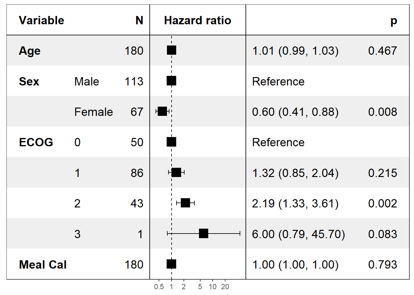

Meta-analysis forest plot

Tips to read

each line corresponds to a study
the symbol (here square or diamond) corresponds to the estimate of the parameter studied (here a relative risk)
the size of the symbol is proportional to the precision
the vertical bar is the value of the parameter in the absence of effect (here 1 because it is a relative risk)
the horizontal bars correspond to the confidence interval of the reported parameter (here the relative risk)
if the symbol is on the right of the vertical line, it means that the link between the treatment (here inspiratory muscle training) and the endpoint (here survival) is positive
if the symbol is to the left of the vertical line, it means that the link between the treatment (here inspiratory muscle training) and the endpoint (here survival) is negative
if the horizontal bar crosses the vertical bar then the link is not significant
the diamond represents the parameter estimated from all the studies

library(forestplot)
library(tibble)
library(tidyjson)
library(dplyr)

# Cochrane data
base_data <- tibble(mean  = c(0.578, 0.165, 0.246, 0.700, 0.348, 0.139, 1.017), 
                    lower = c(0.372, 0.018, 0.072, 0.333, 0.083, 0.016, 0.365),
                    upper = c(0.898, 1.517, 0.833, 1.474, 1.455, 1.209, 2.831),
                    study = c("Auckland", "Block", "Doran", "Gamsu", "Morrison", "Papageorgiou", "Tauesch"),
                    deaths_steroid = c("36", "1", "4", "14", "3", "1", "8"),
                    deaths_placebo = c("60", "5", "11", "20", "7", "7", "10"),
                    OR = c("0.58", "0.16", "0.25", "0.70", "0.35", "0.14", "1.02"))

summary <- tibble(mean  = 0.531, 
                  lower = 0.386,
                  upper = 0.731,
                  study = "Summary",
                  OR = "0.53",
                  summary = TRUE)

header <- tibble(study = c("", "Study"),
                 deaths_steroid = c("Deaths", "(steroid)"),
                 deaths_placebo = c("Deaths", "(placebo)"),
                 OR = c("", "OR"),
                 summary = TRUE)

empty_row <- tibble(mean = NA_real_)

cochrane_output_df <- bind_rows(header,
                                base_data,
                                empty_row,
                                summary)

cochrane_output_df %>% 
  forestplot(labeltext = c(study, deaths_steroid, deaths_placebo, OR), 
             is.summary = summary,
             clip = c(0.1, 2.5), 
             hrzl_lines = list("3" = gpar(lty = 2), 
                               "11" = gpar(lwd = 1, columns = 1:4, col = "#000044")),
             xlog = TRUE,
             col = fpColors(box = "royalblue",
                            line = "darkblue", 
                            summary = "royalblue",
                            hrz_lines = "#444444"))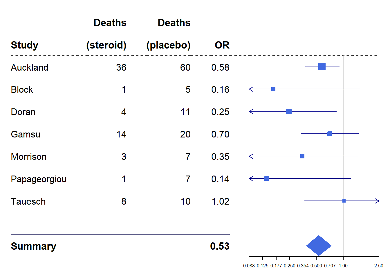

Contact

This document is a work by Emma Lafaurie (emma.lafaurie@inserm.fr) for the SBIM (Service de Biostatistique et Information Médicale) at Saint-Louis Hospital in Paris.
Based on the template of Yan Holtz.

Github SBIM